Simulation Scheme: There are 128 sensors evenly spaced. Width of each sensor is 0.27 mm and empty space between each sensor is 0.03 mm. We assume that there is no attenuation. Image has 50 mm depth(in z direction) and 38 mm width(in x direction). Bubble density is chosen as 260 bubbles per cm2. Transducer frequency is 5 Mhz. There is one single plane wave. Pixel sizes are \( \frac{ \lambda}{8} =0.0385 mm\) in x direction and \( \frac{ \lambda}{20} = 0.0154mm \) in z direction. Total number of pixels in x direction is 990 and total pixels in z direction is 3247.
Training process: Training is done using patches. Lets have some definitions as follows:
x: a patch form ground truth image ( \( 64pixels\times 64pixels \)) ( \(1.97mm \times 4.8mm\) )
y: a patch form Field2 simulation image ( \( 128pixels\times 128pixels \)) (\(1.97mm \times 4.8mm\))
z: output of the network
f : blur kernel (Gaussian kernel with sigma=2 in pixel coordinates)
\[ w = z * f \]
\[ v = x*f \]
Then the training lost can be expressed as follows:
\[ loss = MSEloss(z-v) + \lambda \times L1loss(z)\]
stepsize = 2e-5
\[ \lambda = 0.01\]
Network Structure: Our network is based U-Net with batch normalization and drop out layer. This network is less complex than previous blog. This has 4 convolution layers and 2 ConvTranspose2d layers. Previosuly, there were 9 conv layers and 4 ConvTranspose2d layers.
RESULTS
Note: In all loss graphs, the first losses are eliminated since first training losses are generally huge. By doing that, we can see the behavior better.
Training without label:
The following results for training separately;
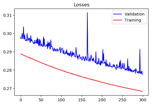
Region 1:
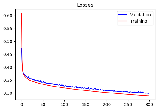
Training Loss at epoch 300 = 0.2890015015956882
Test Loss at epoch 300 = 0.29816133504502274
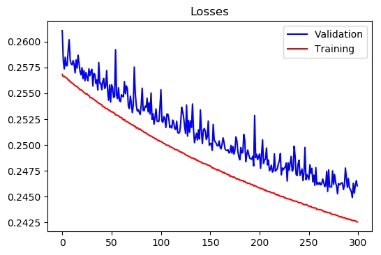
Region 2:
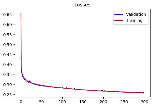
Training Loss at epoch 300 = 0.2568222934655938
Test Loss at epoch 300= 0.25886474471957505
Region 3:
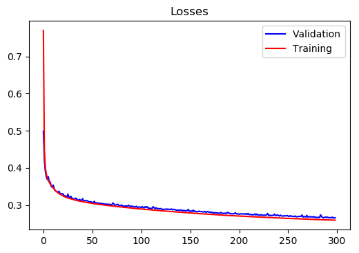
Training Loss at epoch 300= 0.2593389457491914
Test Loss at epoch 300= 0.26586996857076883
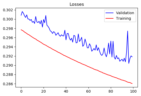
Training with all regions;
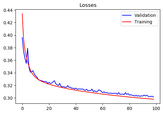
Training Loss at epoch 100= 0.2978930800563814
Test Loss at epoch 100= 0.3013238058236837
Improvement coming from using three different networks instead of one network is more than %9. It is calculated as follows:
\[ Improvement = \frac{ \frac{PatchNumber1*Test Loss1 + PatchNumber2*Test Loss2 + PatchNumber3* Test Loss3 }{TotalPatch} }{Test LossAll} \]
Training without label 2:
The following results are continuation of previous results.
Region 1:
Training Loss at epoch 600 = 0.26843295202074496
Test Loss at epoch 600 = 0.2775525359513926
Region 2:
Training Loss at epoch 600 = 0.24256060957564454
Test Loss at epoch 600= 0.24605255386264455
Region 3:

Training Loss at epoch 600= 0.2436071349660945
Test Loss at epoch 600= 0.2502811230512129
Training with all regions;
Training Loss at epoch 200= 0.2860249894863928
Test Loss at epoch 200= 0.29182279608363587